Last updated: 2026-01-06
Checks: 7 0
Knit directory: DXR_website/
This reproducible R Markdown analysis was created with workflowr (version 1.7.1). The Checks tab describes the reproducibility checks that were applied when the results were created. The Past versions tab lists the development history.
Great! Since the R Markdown file has been committed to the Git repository, you know the exact version of the code that produced these results.
Great job! The global environment was empty. Objects defined in the global environment can affect the analysis in your R Markdown file in unknown ways. For reproduciblity it’s best to always run the code in an empty environment.
The command set.seed(20251201) was run prior to running
the code in the R Markdown file. Setting a seed ensures that any results
that rely on randomness, e.g. subsampling or permutations, are
reproducible.
Great job! Recording the operating system, R version, and package versions is critical for reproducibility.
Nice! There were no cached chunks for this analysis, so you can be confident that you successfully produced the results during this run.
Great job! Using relative paths to the files within your workflowr project makes it easier to run your code on other machines.
Great! You are using Git for version control. Tracking code development and connecting the code version to the results is critical for reproducibility.
The results in this page were generated with repository version e4705f6. See the Past versions tab to see a history of the changes made to the R Markdown and HTML files.
Note that you need to be careful to ensure that all relevant files for
the analysis have been committed to Git prior to generating the results
(you can use wflow_publish or
wflow_git_commit). workflowr only checks the R Markdown
file, but you know if there are other scripts or data files that it
depends on. Below is the status of the Git repository when the results
were generated:
Ignored files:
    Ignored:    .Rhistory
    Ignored:    .Rproj.user/
    Ignored:    DXR_website/data/
    Ignored:    code/Flow_Purity_Stressor_Boxplots_EMP_250226.R
    Ignored:    data/CDKN1A_geneplot_Dox.RDS
    Ignored:    data/Cormotif_dox.RDS
    Ignored:    data/Cormotif_prob_gene_list.RDS
    Ignored:    data/Cormotif_prob_gene_list_doxonly.RDS
    Ignored:    data/Counts_RNA_EMPfortmiller.txt
    Ignored:    data/DMSO_TNN13_plot.RDS
    Ignored:    data/DOX_TNN13_plot.RDS
    Ignored:    data/DOXgeneplots.RDS
    Ignored:    data/ExpressionMatrix_EMP.csv
    Ignored:    data/Ind1_DOX_Spearman_plot.RDS
    Ignored:    data/Ind6REP_Spearman_list.csv
    Ignored:    data/Ind6REP_Spearman_plot.RDS
    Ignored:    data/Ind6REP_Spearman_set.csv
    Ignored:    data/Ind6_Spearman_plot.RDS
    Ignored:    data/MDM2_geneplot_Dox.RDS
    Ignored:    data/Master_summary_75-1_EMP_250811_final.csv
    Ignored:    data/Master_summary_87-1_EMP_250811_final.csv
    Ignored:    data/Metadata.csv
    Ignored:    data/Metadata_2_norep_update.RDS
    Ignored:    data/Metadata_update.csv
    Ignored:    data/QC/
    Ignored:    data/Recovery_flow_purity.csv
    Ignored:    data/SIRT1_geneplot_Dox.RDS
    Ignored:    data/Sample_annotated.csv
    Ignored:    data/SpearmanHeatmapMatrix_EMP
    Ignored:    data/VolcanoPlot_D144R_original_EMP_250623.png
    Ignored:    data/VolcanoPlot_D24R_original_EMP_250623.png
    Ignored:    data/VolcanoPlot_D24T_original_EMP_250623.png
    Ignored:    data/annot_dox.RDS
    Ignored:    data/annot_list_hm.csv
    Ignored:    data/cormotif_dxr_1.RDS
    Ignored:    data/cormotif_dxr_2.RDS
    Ignored:    data/counts/
    Ignored:    data/counts_DE_df_dox.RDS
    Ignored:    data/counts_DE_raw_data.RDS
    Ignored:    data/counts_raw_filt.RDS
    Ignored:    data/counts_raw_matrix.RDS
    Ignored:    data/counts_raw_matrix_EMP_250514.csv
    Ignored:    data/d24_Spearman_plot.RDS
    Ignored:    data/dge_calc_dxr.RDS
    Ignored:    data/dge_calc_matrix.RDS
    Ignored:    data/ensembl_backup_dox.RDS
    Ignored:    data/fC_AllCounts.RDS
    Ignored:    data/fC_DOXCounts.RDS
    Ignored:    data/featureCounts_Concat_Matrix_DOXSamples_EMP_250430.csv
    Ignored:    data/featureCounts_DOXdata_updatedind.RDS
    Ignored:    data/filcpm_colnames_matrix.csv
    Ignored:    data/filcpm_matrix.csv
    Ignored:    data/filt_gene_list_dox.RDS
    Ignored:    data/filter_gene_list_final.RDS
    Ignored:    data/final_data/
    Ignored:    data/gene_clustlike_motif.RDS
    Ignored:    data/gene_postprob_motif.RDS
    Ignored:    data/genedf_dxr.RDS
    Ignored:    data/genematrix_dox.RDS
    Ignored:    data/genematrix_dxr.RDS
    Ignored:    data/heartgenes.csv
    Ignored:    data/heartgenes_dox.csv
    Ignored:    data/image_intensity_stats_all_conditions.csv
    Ignored:    data/image_level_stats_all_conditions.csv
    Ignored:    data/image_level_summary_yH2AX_quant.csv
    Ignored:    data/ind_num_dox.RDS
    Ignored:    data/ind_num_dxr.RDS
    Ignored:    data/initial_cormotif.RDS
    Ignored:    data/initial_cormotif_dox.RDS
    Ignored:    data/low_nuclei_samples.csv
    Ignored:    data/low_veh_samples.csv
    Ignored:    data/new/
    Ignored:    data/new_cormotif_dox.RDS
    Ignored:    data/perc_mean_all_10X.png
    Ignored:    data/perc_mean_all_20X.png
    Ignored:    data/perc_mean_all_40X.png
    Ignored:    data/perc_mean_consistent_10X.png
    Ignored:    data/perc_mean_consistent_20X.png
    Ignored:    data/perc_mean_consistent_40X.png
    Ignored:    data/perc_median_all_10X.png
    Ignored:    data/perc_median_all_20X.png
    Ignored:    data/perc_median_all_40X.png
    Ignored:    data/perc_median_consistent_10X.png
    Ignored:    data/perc_median_consistent_20X.png
    Ignored:    data/perc_median_consistent_40X.png
    Ignored:    data/plot_leg_d.RDS
    Ignored:    data/plot_leg_d_horizontal.RDS
    Ignored:    data/plot_leg_d_vertical.RDS
    Ignored:    data/plot_theme_custom.RDS
    Ignored:    data/process_gene_data_funct.RDS
    Ignored:    data/raw_mean_all_10X.png
    Ignored:    data/raw_mean_all_20X.png
    Ignored:    data/raw_mean_all_40X.png
    Ignored:    data/raw_mean_consistent_10X.png
    Ignored:    data/raw_mean_consistent_20X.png
    Ignored:    data/raw_mean_consistent_40X.png
    Ignored:    data/raw_median_all_10X.png
    Ignored:    data/raw_median_all_20X.png
    Ignored:    data/raw_median_all_40X.png
    Ignored:    data/raw_median_consistent_10X.png
    Ignored:    data/raw_median_consistent_20X.png
    Ignored:    data/raw_median_consistent_40X.png
    Ignored:    data/ruv/
    Ignored:    data/summary_all_IF_ROI.RDS
    Ignored:    data/tableED_GOBP.RDS
    Ignored:    data/tableESR_GOBP_postprob.RDS
    Ignored:    data/tableLD_GOBP.RDS
    Ignored:    data/tableLR_GOBP_postprob.RDS
    Ignored:    data/tableNR_GOBP.RDS
    Ignored:    data/tableNR_GOBP_postprob.RDS
    Ignored:    data/table_incsus_genes_GOBP_RUV.RDS
    Ignored:    data/table_motif1_GOBP_d.RDS
    Ignored:    data/table_motif1_genes_GOBP.RDS
    Ignored:    data/table_motif2_GOBP_d.RDS
    Ignored:    data/table_motif3_genes_GOBP.RDS
    Ignored:    data/thing.R
    Ignored:    data/top.table_V.D144r_dox.RDS
    Ignored:    data/top.table_V.D24_dox.RDS
    Ignored:    data/top.table_V.D24r_dox.RDS
    Ignored:    data/yH2AX_75-1_EMP_250811.csv
    Ignored:    data/yH2AX_87-1_EMP_250811.csv
    Ignored:    data/yH2AX_Boxplots_MeanIntensity_10X_EMP_250811.png
    Ignored:    data/yH2AX_Boxplots_MeanIntensity_10X_NormtoMax_EMP_250811.png
    Ignored:    data/yH2AX_Boxplots_MeanIntensity_20X_EMP_250811.png
    Ignored:    data/yH2AX_Boxplots_MeanIntensity_20X_NormtoMax_EMP_250811.png
    Ignored:    data/yH2AX_Boxplots_MedianIntensity_10X_NormtoMax_EMP_250811.png
    Ignored:    data/yH2AX_Boxplots_MedianIntensity_20X_NormtoMax_EMP_250811.png
    Ignored:    data/yH2AX_Boxplots_MedianIntensity_NormtoMax_EMP_250811.png
    Ignored:    data/yH2AX_Boxplots_Quant_10X_EMP_250817.png
    Ignored:    data/yH2AX_Boxplots_Quant_20X_EMP_250817.png
    Ignored:    data/yh2ax_all_df_EMP_250812.csv
Note that any generated files, e.g. HTML, png, CSS, etc., are not included in this status report because it is ok for generated content to have uncommitted changes.
These are the previous versions of the repository in which changes were
made to the R Markdown (DXR_website/analysis/QC.Rmd) and
HTML (DXR_website/docs/QC.html) files. If you’ve configured
a remote Git repository (see ?wflow_git_remote), click on
the hyperlinks in the table below to view the files as they were in that
past version.
| File | Version | Author | Date | Message |
|---|---|---|---|---|
| html | c382b38 | emmapfort | 2026-01-06 | Build site. |
| Rmd | cd535e9 | emmapfort | 2026-01-06 | Final Website Touches 01/06/25 EMP |
| html | 7f22593 | emmapfort | 2026-01-05 | Build site. |
| html | f088a00 | emmapfort | 2025-12-09 | website updates |
| Rmd | a967d53 | emmapfort | 2025-12-09 | Update website and analysis chunks |
| html | a967d53 | emmapfort | 2025-12-09 | Update website and analysis chunks |
| Rmd | da1f69c | emmapfort | 2025-12-02 | updated analysis 12/02/25 |
Libraries
Load necessary libraries for analysis.
library(tidyverse)
library(readr)
library(readxl)
library(edgeR)
library(ggfortify)
library(ComplexHeatmap)
library(ggrepel)
Define my custom plot theme
# Define the custom theme
# plot_theme_custom <- function() {
#   theme_minimal() +
#     theme(
#       #line for x and y axis
#       axis.line = element_line(linewidth = 1,
#                                color = "black"),
#
#       #axis ticks only on x and y, length standard
#       axis.ticks.x = element_line(color = "black",
#                                 linewidth = 1),
#       axis.ticks.y = element_line(color = "black",
#                                 linewidth = 1),
#       axis.ticks.length = unit(0.05, "in"),
#
#       #text and font
#       axis.text = element_text(color = "black",
#                                family = "Arial",
#                                size = 7),
#       axis.title = element_text(color = "black",
#                                 family = "Arial",
#                                 size = 9),
#       legend.text = element_text(color = "black",
#                                  family = "Arial",
#                                  size = 7),
#       legend.title = element_text(color = "black",
#                                   family = "Arial",
#                                   size = 9),
#       plot.title = element_text(color = "black",
#                                 family = "Arial",
#                                 size = 10),
#
#       #blank background and border
#       panel.background = element_blank(),
#       panel.border = element_blank(),
#
#       #gridlines for alignment
#       panel.grid.major = element_line(color = "grey80", linewidth = 0.5),  #grey major grid for align in illus
#       panel.grid.minor = element_line(color = "grey90", linewidth = 0.5) #grey minor grid for align in illus
#     )
# }

# saveRDS(plot_theme_custom, "data/plot_theme_custom.RDS")

theme_custom <- readRDS("data/plot_theme_custom.RDS")
Define a function to save plots as .pdf and .png
save_plot <- function(plot, filename,
                      folder = ".",
                      width = 8,
                      height = 6,
                      units = "in",
                      dpi = 300,
                      add_date = TRUE) {
  if (missing(filename)) stop("Please provide a filename (without extension) for the plot.")

  date_str <- if (add_date) paste0("_", format(Sys.Date(), "%y%m%d")) else ""
  pdf_file <- file.path(folder, paste0(filename, date_str, ".pdf"))
  png_file <- file.path(folder, paste0(filename, date_str, ".png"))
  ggsave(filename = pdf_file, plot = plot, device = cairo_pdf, width = width, height = height, units = units, bg = "transparent")
  ggsave(filename = png_file, plot = plot, device = "png", width = width, height = height, units = units, dpi = dpi, bg = "transparent")
  message("Saved plot as Cairo PDF: ", pdf_file)
  message("Saved plot as PNG: ", png_file)
}

output_folder <- "C:/Users/emmap/OneDrive/Desktop/DXR Manuscript Materials/Fig pdfs"


#save plot function created
#to use: just define the plot name, filename_base, width, height
Initial Dataframes
Create the initial dataframes from counts files needed to start analysis.
Read in Counts Files from FeatureCounts
#load in libraries needed
#these counts files are from featureCounts, all saved as RDS objects

#prev Ind1 84-1 is now Ind4

# ####Individual 1 - 87-1####
# Counts_87_DOX_24 <- readRDS("data/QC/Counts_87_DOX_24.RDS")
# Counts_87_DMSO_24 <- readRDS("data/QC/Counts_87_DMSO_24.RDS")
# Counts_87_DOX_24rec <- readRDS("data/QC/Counts_87_DOX_24rec.RDS")
# Counts_87_DMSO_24rec <- readRDS("data/QC/Counts_87_DMSO_24rec.RDS")
# Counts_87_DOX_144rec <- readRDS("data/QC/Counts_87_DOX_144rec.RDS")
# Counts_87_DMSO_144rec <- readRDS("data/QC/Counts_87_DMSO_144rec.RDS")
#
# ####Individual 2 - 78-1####
# Counts_78_DOX_24 <- readRDS("data/QC/Counts_78_DOX_24.RDS")
# Counts_78_DMSO_24 <- readRDS("data/QC/Counts_78_DMSO_24.RDS")
# Counts_78_DOX_24rec <- readRDS("data/QC/Counts_78_DOX_24rec.RDS")
# Counts_78_DMSO_24rec <- readRDS("data/QC/Counts_78_DMSO_24rec.RDS")
# Counts_78_DOX_144rec <- readRDS("data/QC/Counts_78_DOX_144rec.RDS")
# Counts_78_DMSO_144rec <- readRDS("data/QC/Counts_78_DMSO_144rec.RDS")
#
# ####Individual 3 - 75-1####
# Counts_75_DOX_24 <- readRDS("data/QC/Counts_75_DOX_24.RDS")
# Counts_75_DMSO_24 <- readRDS("data/QC/Counts_75_DMSO_24.RDS")
# Counts_75_DOX_24rec <- readRDS("data/QC/Counts_75_DOX_24rec.RDS")
# Counts_75_DMSO_24rec <- readRDS("data/QC/Counts_75_DMSO_24rec.RDS")
# Counts_75_DOX_144rec <- readRDS("data/QC/Counts_75_DOX_144rec.RDS")
# Counts_75_DMSO_144rec <- readRDS("data/QC/Counts_75_DMSO_144rec.RDS")
#
# ####Individual 4 - 84-1####
# Counts_84_DOX_24 <- readRDS("data/QC/Counts_84_DOX_24.RDS")
# Counts_84_DMSO_24 <- readRDS("data/QC/Counts_84_DMSO_24.RDS")
# Counts_84_DOX_24rec <- readRDS("data/QC/Counts_84_DOX_24rec.RDS")
# Counts_84_DMSO_24rec <- readRDS("data/QC/Counts_84_DMSO_24rec.RDS")
# Counts_84_DOX_144rec <- readRDS("data/QC/Counts_84_DOX_144rec.RDS")
# Counts_84_DMSO_144rec <- readRDS("data/QC/Counts_84_DMSO_144rec.RDS")
#
# ####Individual 5 - 17-3####
# Counts_17_DOX_24 <- readRDS("data/QC/Counts_17_DOX_24.RDS")
# Counts_17_DMSO_24 <- readRDS("data/QC/Counts_17_DMSO_24.RDS")
# Counts_17_DOX_24rec <- readRDS("data/QC/Counts_17_DOX_24rec.RDS")
# Counts_17_DMSO_24rec <- readRDS("data/QC/Counts_17_DMSO_24rec.RDS")
# Counts_17_DOX_144rec <- readRDS("data/QC/Counts_17_DOX_144rec.RDS")
# Counts_17_DMSO_144rec <- readRDS("data/QC/Counts_17_DMSO_144rec.RDS")
#
# ####Individual 6 - 90-1####
# Counts_90_DOX_24 <- readRDS("data/QC/Counts_90_DOX_24.RDS")
# Counts_90_DMSO_24 <- readRDS("data/QC/Counts_90_DMSO_24.RDS")
# Counts_90_DOX_24rec <- readRDS("data/QC/Counts_90_DOX_24rec.RDS")
# Counts_90_DMSO_24rec <- readRDS("data/QC/Counts_90_DMSO_24rec.RDS")
# Counts_90_DOX_144rec <- readRDS("data/QC/Counts_90_DOX_144rec.RDS")
# Counts_90_DMSO_144rec <- readRDS("data/QC/Counts_90_DMSO_144rec.RDS")
#
# ####Individual 7 - 90-1REP####
# Counts_90REP_DOX_24 <- readRDS("data/QC/Counts_90REP_DOX_24.RDS")
# Counts_90REP_DMSO_24 <- readRDS("data/QC/Counts_90REP_DMSO_24.RDS")
# Counts_90REP_DOX_24rec <- readRDS("data/QC/Counts_90REP_DOX_24rec.RDS")
# Counts_90REP_DMSO_24rec <- readRDS("data/QC/Counts_90REP_DMSO_24rec.RDS")
# Counts_90REP_DOX_144rec <- readRDS("data/QC/Counts_90REP_DOX_144rec.RDS")
# Counts_90REP_DMSO_144rec <- readRDS("data/QC/Counts_90REP_DMSO_144rec.RDS")
Create my Dataframe from Counts Files
Combine all of my counts files above into one dataframe, then convert to a matrix for further analysis.
#change 84-1 to Ind4 now

# counts_raw_df <-
#    data.frame(
#      Counts_87_DOX_24,
#      Counts_87_DMSO_24$MCW_EMP_JT_R38_R1.bam,
#      Counts_87_DOX_24rec$MCW_EMP_JT_R39_R1.bam,
#      Counts_87_DMSO_24rec$MCW_EMP_JT_R41_R1.bam,
#      Counts_87_DOX_144rec$MCW_EMP_JT_R42_R1.bam,
#      Counts_87_DMSO_144rec$MCW_EMP_JT_R44_R1.bam,
#      Counts_78_DOX_24$MCW_EMP_JT_R45_R1.bam,
#      Counts_78_DMSO_24$MCW_EMP_JT_R47_R1.bam,
#      Counts_78_DOX_24rec$MCW_EMP_JT_R48_R1.bam,
#      Counts_78_DMSO_24rec$MCW_EMP_JT_R50_R1.bam,
#      Counts_78_DOX_144rec$MCW_EMP_JT_R51_R1.bam,
#      Counts_78_DMSO_144rec$MCW_EMP_JT_R53_R1.bam,
#      Counts_75_DOX_24$MCW_EMP_JT_R54_R1.bam,
#      Counts_75_DMSO_24$MCW_EMP_JT_R56_R1.bam,
#      Counts_75_DOX_24rec$MCW_EMP_JT_R57_R1.bam,
#      Counts_75_DMSO_24rec$MCW_EMP_JT_R59_R1.bam,
#      Counts_75_DOX_144rec$MCW_EMP_JT_R60_R1.bam,
#      Counts_75_DMSO_144rec$MCW_EMP_JT_R62_R1.bam,
#      Counts_84_DOX_24$MCW_EMP_JT_R27_R1.bam,
#      Counts_84_DMSO_24$MCW_EMP_JT_R29_R1.bam,
#      Counts_84_DOX_24rec$MCW_EMP_JT_R30_R1.bam,
#      Counts_84_DMSO_24rec$MCW_EMP_JT_R32_R1.bam,
#      Counts_84_DOX_144rec$MCW_EMP_JT_R33_R1.bam,
#      Counts_84_DMSO_144rec$MCW_EMP_JT_R35_R1.bam,
#      Counts_17_DOX_24$MCW_EMP_JT_R63_R1.bam,
#      Counts_17_DMSO_24$MCW_EMP_JT_R65_R1.bam,
#      Counts_17_DOX_24rec$MCW_EMP_JT_R66_R1.bam,
#      Counts_17_DMSO_24rec$MCW_EMP_JT_R68_R1.bam,
#      Counts_17_DOX_144rec$MCW_EMP_JT_R69_R1.bam,
#      Counts_17_DMSO_144rec$MCW_EMP_JT_R71_R1.bam,
#      Counts_90_DOX_24$MCW_EMP_JT_R72_R1.bam,
#      Counts_90_DMSO_24$MCW_EMP_JT_R74_R1.bam,
#      Counts_90_DOX_24rec$MCW_EMP_JT_R75_R1.bam,
#      Counts_90_DMSO_24rec$MCW_EMP_JT_R77_R1.bam,
#      Counts_90_DOX_144rec$MCW_EMP_JT_R78_R1.bam,
#      Counts_90_DMSO_144rec$MCW_EMP_JT_R80_R1.bam,
#      Counts_90REP_DOX_24$MCW_EMP_JT_R81_R1.bam,
#      Counts_90REP_DMSO_24$MCW_EMP_JT_R83_R1.bam,
#      Counts_90REP_DOX_24rec$MCW_EMP_JT_R84_R1.bam,
#      Counts_90REP_DMSO_24rec$MCW_EMP_JT_R86_R1.bam,
#      Counts_90REP_DOX_144rec$MCW_EMP_JT_R87_R1.bam,
#      Counts_90REP_DMSO_144rec$MCW_EMP_JT_R89_R1.bam
#    )

# saveRDS(counts_raw_df, "data/QC/counts_raw_df.RDS")

#now convert this into a matrix
# counts_raw_matrix <- counts_raw_df %>% column_to_rownames(var = "X") %>% as.matrix()

#write this to a csv so I can save it for later
# write.csv(counts_raw_matrix, "data/QC/counts_raw_matrix.csv")

#I also want to save this as an R object so I don't have to run the counts every time
# saveRDS(counts_raw_matrix, "data/QC/counts_raw_matrix.RDS")

counts_raw_matrix <- readRDS("data/QC/counts_raw_matrix.RDS")

dim(counts_raw_matrix)
[1] 28395 42#28395 is my initial amount of genes prior to filteringFactors and Colors
Include each of the factors for these experiments as well as their color schemes.
####Colors####

# txtime_col_old <- list(
#   "DOX_24T" = "#263CA5",
#   "VEH_24T" = "#444343",
#   "DOX_24R" = "#5B8FD1",
#   "VEH_24R" = "#757575",
#   "DOX_144R" = "#89C5E5",
#   "VEH_144R" = "#AAAAAA"
# )

#updated colors and factors:
ind_col <- list(
  "1" = "#FF9F64",
  "2" = "#78EBDA",
  "3" = "#ADCD77",
  "4" = "#E6CC50",
  "5" = "#A68AC0",
  "6" = "#F16F90",
  "6R" = "#C61E4E"
)

ind_col_nr <- list(
  "1" = "#FF9F64",
  "2" = "#78EBDA",
  "3" = "#ADCD77",
  "4" = "#E6CC50",
  "5" = "#A68AC0",
  "6" = "#F16F90"
)

time_col <- list(
  "t0" = "#005A4C",
  "t24" = "#328477",
  "t144" = "#8FB9B1")

tx_col <- list(
  "DOX" = "#499FBD",
  "VEH" = "#BBBBBC")

txtime_col <- list(
  "DOX_t0" = "#263CA5",
  "VEH_t0" = "#444343",
  "DOX_t24" = "#5B8FD1",
  "VEH_t24" = "#757575",
  "DOX_t144" = "#89C5E5",
  "VEH_t144" = "#AAAAAA"
)
QC Mapping Plots
Assess the alignment of each sample to hg38 as performed in command line previously.
Set up initial dataframe
#this dataframe contains my alignment percentages from featureCounts

#I originally had fC_DOXCounts which contained the individuals prior to their final order - here is the code that I used to change it

#I want to change these to reflect the final order of samples
# fC_DOXCounts <- fC_DOXCounts %>%
#   mutate(
#     Ind = case_when(
#       Line == "87-1" ~ "1",
#       Line == "78-1" ~ "2",
#       Line == "75-1" ~ "3",
#       Line == "84-1" ~ "4",
#       Line == "17-3" ~ "5",
#       Line == "90-1" ~ "6",
#       Line == "90-1REP" ~ "6R",
#       TRUE ~ NA_character_
#     ),
#   Tx = ifelse(Treatment == "DMSO", "VEH", "DOX"),
#   Timepoint = case_when(
#     Time == "24" ~ "t0",
#     Time == "24rec" ~ "t24",
#     Time == "144rec" ~ "t144",
#     TRUE ~ NA_character_
#                      ),
#     Condition = paste0(Tx, "_", Timepoint, "_", Ind)
#   )
#
# #factor individual
# fC_DOXCounts <- fC_DOXCounts %>%
#   mutate(
#     Ind = factor(Ind, levels = c("1", "2", "3", "4", "5", "6", "6R"),
#                  ordered = TRUE)
#   )
#
#
# fC_DOXCounts <- fC_DOXCounts %>%
#   mutate(
#     Ind = factor(Ind, levels = c("1", "2", "3", "4", "5", "6", "6R"),
#                  ordered = TRUE),
#         Timepoint = factor(Timepoint, levels = c("t0", "t24", "t144"),
#                        ordered = TRUE),
#         Tx = factor(Tx, levels = c("DOX", "VEH"),
#                     ordered = TRUE)
#   ) %>%
#   mutate(
#     Condition = factor(
#       Condition,
#       levels = expand.grid(
#         Tx = levels(Tx),
#         Timepoint = levels(Timepoint),
#         Ind = levels(Ind)
#       ) %>%
#         transmute(Condition = paste(Tx, Timepoint, Ind, sep = "_")) %>%
#         pull(Condition),
#       ordered = TRUE
#     )
#   )

# saveRDS(fC_DOXCounts, "data/QC/featureCounts_DOXdata_updatedind.RDS")


fC_DOXCounts <- readRDS("data/QC/featureCounts_DOXdata_updatedind.RDS")

#Now I want to plot these values out
Total Fragments Plots
Assess the total number of fragments for each sample (paired-end reads)
####By Sample####
reads_by_sample <- c("DOX" = "#499FBD", "VEH" = "#BBBBBC")

fC_DOXCounts %>%
  ggplot(., aes (x = Condition,
                 y = Total_Align,
                 fill = Tx,
                 group_by = Ind))+
  geom_col()+
  geom_hline(aes(yintercept = 20000000))+
  scale_fill_manual(values = reads_by_sample)+
  ggtitle(expression("Total fragments by sample"))+
  xlab("")+
  ylab(expression("RNA-sequencing reads"))+
  theme_custom()+
  theme(plot.title = element_text(size = rel(2), hjust = 0.5),
        axis.title = element_text(size = 15, color = "black"),
        axis.ticks = element_line(linewidth = 1.5),
        axis.text.y = element_text(size =10, color = "black", angle = 0, hjust = 0.8, vjust = 0.5),
        axis.text.x = element_text(size =10, color = "black", angle = 90, hjust = 1, vjust = 0.2),
        strip.text.y = element_text(color = "white"))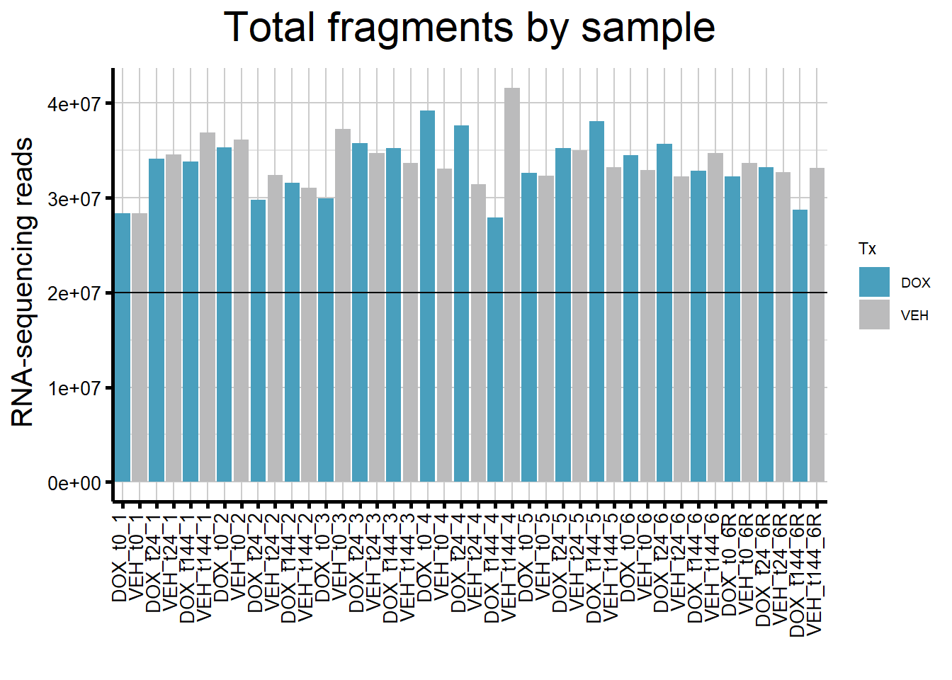
| Version | Author | Date |
|---|---|---|
| a967d53 | emmapfort | 2025-12-09 |
####By Treatment####
fC_DOXCounts %>%
  ggplot(., aes (x = Tx, y= Total_Align, fill = Tx))+
  geom_boxplot()+
 scale_fill_manual(values=reads_by_sample)+
  ggtitle(expression("Total fragments by treatment"))+
  xlab("")+
  ylab(expression("RNA-sequencing reads"))+
  theme_bw()+

  theme(plot.title = element_text(size = rel(2), hjust = 0.5),
        axis.title = element_text(size = 15, color = "black"),
        axis.ticks = element_line(linewidth = 1.5),
        axis.text.y = element_text(size =10, color = "black", angle = 0, hjust = 0.8, vjust = 0.5),
        axis.text.x = element_text(size =10, color = "black", angle = 90, hjust = 1, vjust = 0.2),
        #strip.text.x = element_text(size = 15, color = "black", face = "bold"),
        strip.text.y = element_text(color = "white"))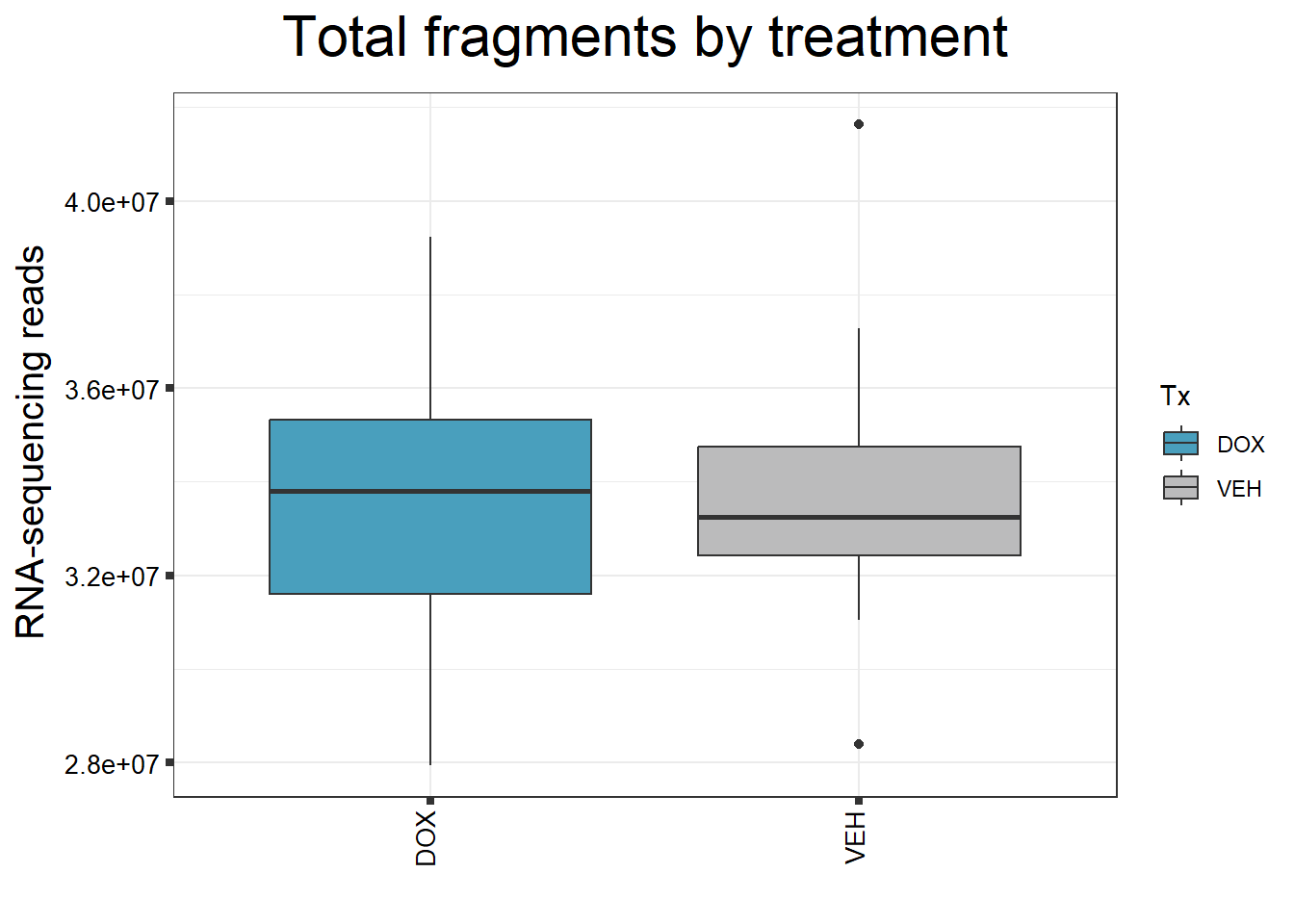
| Version | Author | Date |
|---|---|---|
| a967d53 | emmapfort | 2025-12-09 |
####By Individual####
fC_DOXCounts %>%
  ggplot(., aes (x =as.factor(Ind), y=Total_Align))+
  geom_boxplot(aes(fill=as.factor(Ind)))+
 scale_fill_brewer(palette = "Dark2", name = "Individual")+
  ggtitle(expression("Total fragments by individual"))+
  xlab("")+
  ylab(expression("RNA-sequencing reads"))+
  theme_bw()+

  theme(plot.title = element_text(size = rel(2), hjust = 0.5),
        axis.title = element_text(size = 15, color = "black"),
        axis.ticks = element_line(linewidth = 1.5),
        axis.text.y = element_text(size =10, color = "black", angle = 0, hjust = 0.8, vjust = 0.5),
        axis.text.x = element_text(size =10, color = "black", angle = 0, hjust = 1),
        #strip.text.x = element_text(size = 15, color = "black", face = "bold"),
        strip.text.y = element_text(color = "white"))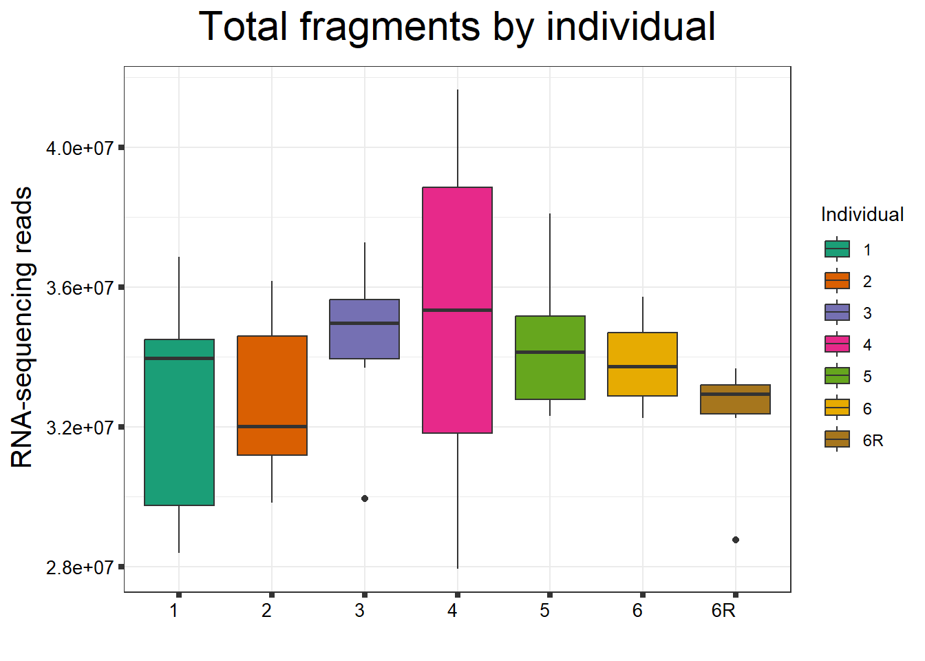
| Version | Author | Date |
|---|---|---|
| a967d53 | emmapfort | 2025-12-09 |
####By Timepoint####
reads_by_time <- c("t0" = "#005A4C",
                 "t24" = "#328477",
                 "t144" = "#8FB9B1")

fC_DOXCounts$Time <- factor(fC_DOXCounts$Time,
                            levels = c("t0", "t24", "t144"))

total_by_time <- fC_DOXCounts %>%
  ggplot(., aes (x = Condition, y = Total_Align,
                 fill = Timepoint, group_by = Ind))+
  geom_col()+
 geom_hline(aes(yintercept=20000000))+
 scale_fill_manual(values=reads_by_time)+
  ggtitle(expression("Total fragments by timepoint"))+
  xlab("")+
  ylab(expression("RNA-sequencing reads"))+
  theme_custom()+
  theme(
        axis.ticks = element_line(linewidth = 1.5),
        axis.text.y = element_text(angle = 0, hjust = 0.8, vjust = 0.5),
        axis.text.x = element_text(angle = 90, hjust = 1, vjust = 0.2),
        strip.text.y = element_text(color = "white"))


####By Individual####
fC_DOXCounts %>%
  ggplot(., aes (x =as.factor(Ind), y=Total_Align))+
  geom_boxplot(aes(fill=as.factor(Ind)))+
 scale_fill_brewer(palette = "Dark2", name = "Individual")+
  ggtitle(expression("Total number of mapped reads by individual"))+
  xlab("")+
  ylab(expression("RNA-sequencing reads"))+
  theme_bw()+

  theme(plot.title = element_text(size = rel(2), hjust = 0.5),
        axis.title = element_text(size = 15, color = "black"),
        axis.ticks = element_line(linewidth = 1.5),
        axis.text.y = element_text(size =10, color = "black", angle = 0, hjust = 0.8, vjust = 0.5),
        axis.text.x = element_text(size =10, color = "black", angle = 0, hjust = 1),
        #strip.text.x = element_text(size = 15, color = "black", face = "bold"),
        strip.text.y = element_text(color = "white"))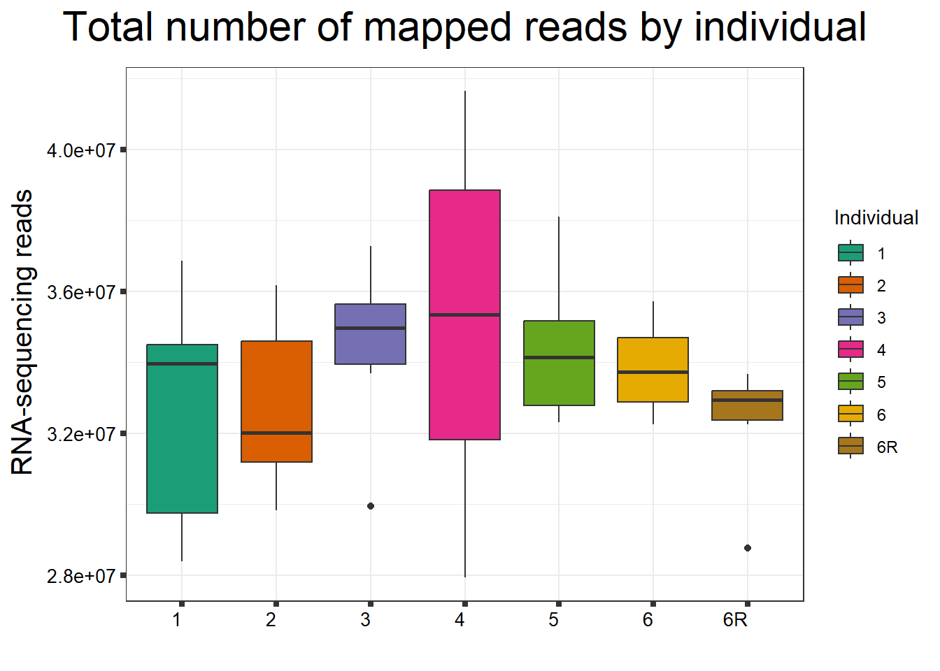
| Version | Author | Date |
|---|---|---|
| a967d53 | emmapfort | 2025-12-09 |
Mapped Fragments
Assess the number of fragments that were mapped.
Supplementary Figure 1A: Mapped fragments by sample
reads_by_sample <- c("DOX" = "#5B8FD1", "VEH" = "#BBBBBC")
map_sample_plot <- fC_DOXCounts %>%
  ggplot(., aes (x = Condition, y = Assigned_Align, fill = Tx,
                 group_by = Ind))+
  geom_col()+
 geom_hline(aes(yintercept=20000000))+
 scale_fill_manual(values=reads_by_sample)+
  ggtitle(expression("Mapped fragments by sample"))+
  xlab("")+
  ylab(expression("RNA-sequencing reads"))+
  theme_custom()+
  theme(
        axis.text.y = element_text(angle = 0, hjust = 0.8, vjust = 0.5),
        axis.text.x = element_text(angle = 90, hjust = 1, vjust = 0.2),
        strip.text.y = element_text(color = "white"))

# save_plot(
#   plot = map_sample_plot,
#   filename = "MappedReads_Sample_Supp1A_EMP_",
#   folder = output_folder,
#   height = 5,
#   width = 8
# )
Supplementary Figure 1B: Mapped Fragments by Treatment
map_tx_bp <- fC_DOXCounts %>%
  ggplot(., aes (x =Tx, y= Assigned_Align, fill = Tx))+
  geom_boxplot()+
 scale_fill_manual(values=reads_by_sample)+
  ggtitle(expression("Mapped fragments by treatment"))+
  xlab("")+
  ylab(expression("RNA-sequencing reads"))+
  theme_custom()+
  theme(axis.text.y = element_text(angle = 0, hjust = 0.8, vjust = 0.5),
        axis.text.x = element_text(angle = 90, hjust = 1, vjust = 0.2),
        strip.text.y = element_text(color = "white"))

# save_plot(plot = map_tx_bp,
#           filename = "MappedReads_Treatment_Supp1B_EMP_",
#           folder = output_folder)
Supplementary Figure 1C: Mapped Fragments by Timepoint
reads_by_time <- c("t0" = "#005A4C",
                 "t24" = "#328477",
                 "t144" = "#8FB9B1")


map_time_box <- fC_DOXCounts %>%
  ggplot(., aes (x = Timepoint, y= Assigned_Align, fill = Timepoint))+
  geom_boxplot()+
 scale_fill_manual(values=reads_by_time)+
  ggtitle(expression("Mapped fragments by timepoint"))+
  xlab("")+
  ylab(expression("RNA-sequencing reads"))+
  theme_custom()+
  theme(axis.ticks = element_line(linewidth = 1),
        axis.text.y = element_text(angle = 0, hjust = 0.8, vjust = 0.5),
        axis.text.x = element_text(angle = 90, hjust = 1, vjust = 0.2),
        strip.text.y = element_text(color = "white"))

# save_plot(plot = map_time_box,
          # filename = "MappedReads_Boxplot_Supp1C_EMP_",
          # folder = output_folder)
Filter Dataframe
Filter my dataframe by converting to log2cpm and filtering out lowly expressed genes.
#transform counts to cpm as a first step
counts_cpm_unfilt <- cpm(counts_raw_matrix, log = TRUE)
dim(counts_cpm_unfilt)
[1] 28395 42# saveRDS(counts_cpm_unfilt, "data/QC/counts_cpm_unfilt.RDS")
#I should have 28395 genes here since this is unfiltered
hist(counts_cpm_unfilt,
main = "Histogram of Unfiltered Counts",
xlab = expression("Log"[2]*" counts-per-million"),
col = 4)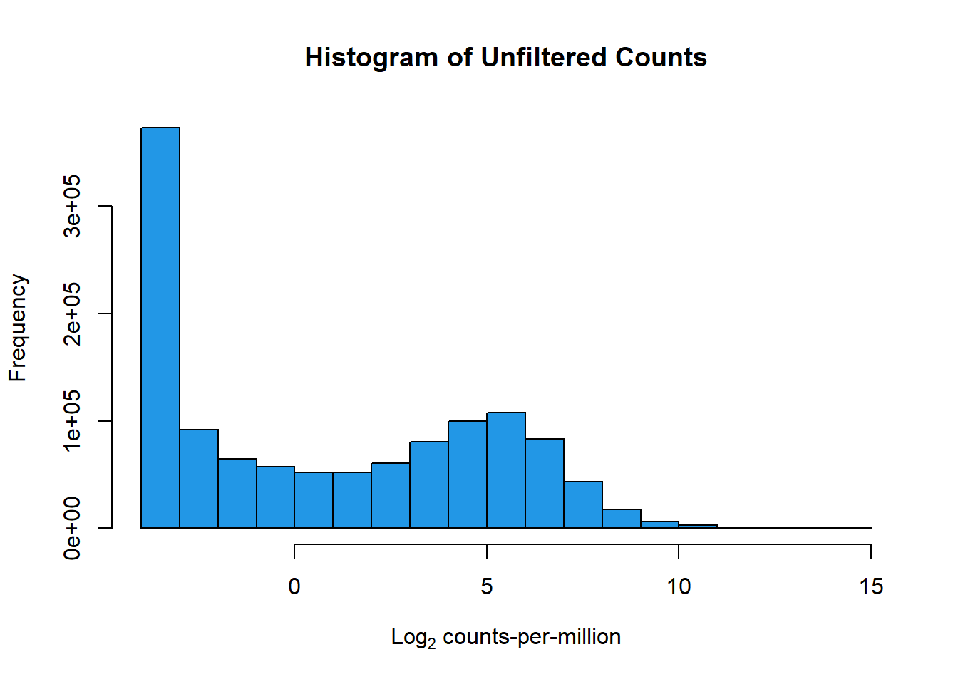
| Version | Author | Date |
|---|---|---|
| a967d53 | emmapfort | 2025-12-09 |
###filter my data by rowMeans > 0 to exclude lowly expressed genes

filcpm_matrix <- subset(counts_cpm_unfilt, (rowMeans(counts_cpm_unfilt) > 0))
dim(filcpm_matrix)
[1] 14319 42#I should have 14319 genes here
#now let's make a histogram of this to check the difference
hist(filcpm_matrix,
main = "Histogram of Filtered Counts by rowMeans > 0",
xlab = expression("Log"[2]*" counts-per-million"),
col = 2)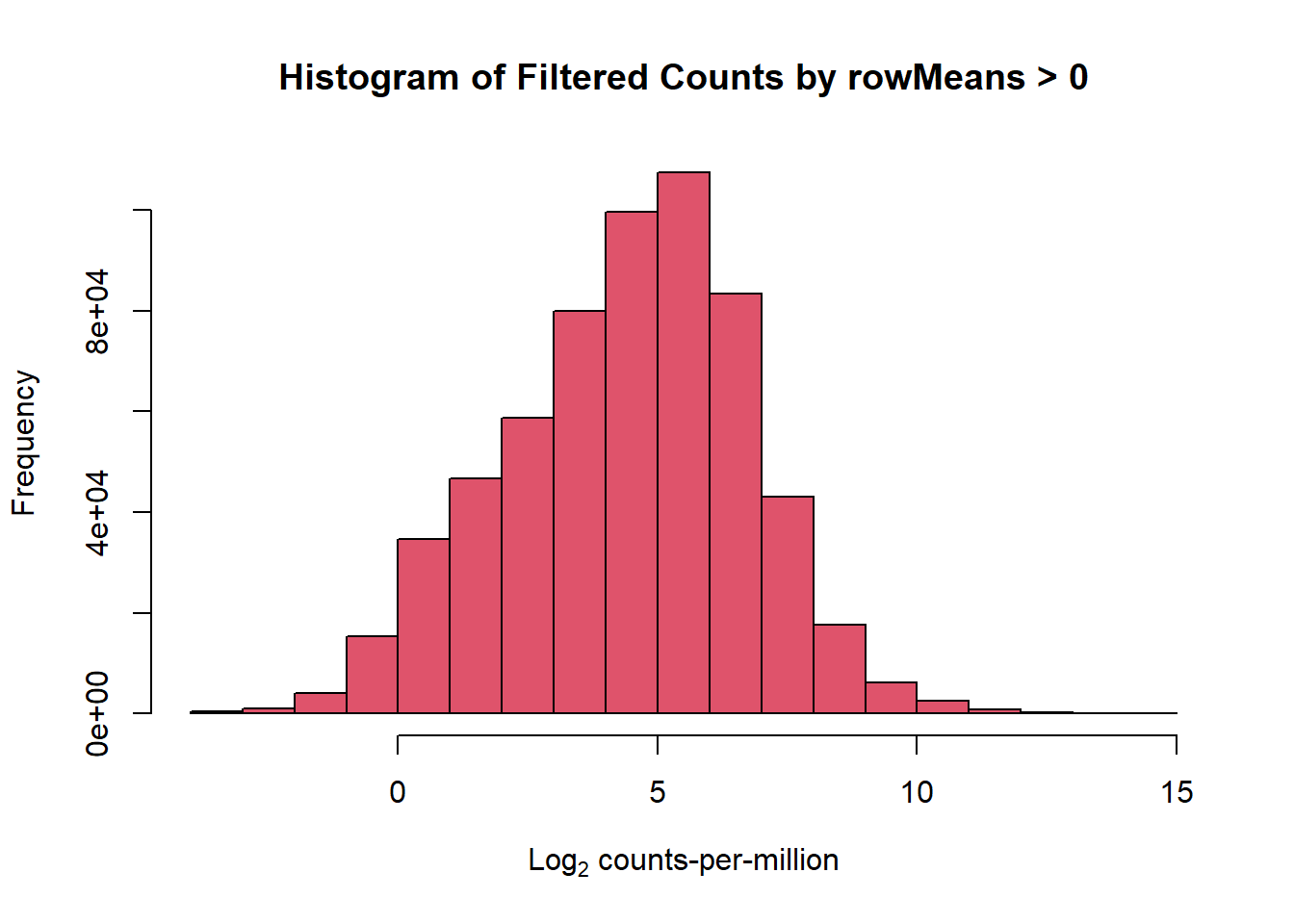
| Version | Author | Date |
|---|---|---|
| a967d53 | emmapfort | 2025-12-09 |
#change the column names to match my samples - make sure that they are in the right order
#Individual 1 = 87-1 (F)
#Individual 2 = 78-1 (F)
#Individual 3 = 75-1 (F)
#Individual 4 = 84-1 (M)
#Individual 5 = 17-3 (M)
#Individual 6 = 90-1 (M)
#Individual 6REP = 90-1REP (M)

#Treatment/time should follow this order:
#DOX24tx
#DMSO24tx
#DOX24rec
#DMSO24rec
#DOX144rec
#DMSO144rec

# colnames(filcpm_matrix) <- c("DOX_24T_Ind1",
#                                 "DMSO_24T_Ind1",
#                                 "DOX_24R_Ind1",
#                                 "DMSO_24R_Ind1",
#                                 "DOX_144R_Ind1",
#                                 "DMSO_144R_Ind1",
#                                 "DOX_24T_Ind2",
#                                 "DMSO_24T_Ind2",
#                                 "DOX_24R_Ind2",
#                                 "DMSO_24R_Ind2",
#                                 "DOX_144R_Ind2",
#                                 "DMSO_144R_Ind2",
#                                 "DOX_24T_Ind3",
#                                 "DMSO_24T_Ind3",
#                                 "DOX_24R_Ind3",
#                                 "DMSO_24R_Ind3",
#                                 "DOX_144R_Ind3",
#                                 "DMSO_144R_Ind3",
#                                 "DOX_24T_Ind4",
#                                 "DMSO_24T_Ind4",
#                                 "DOX_24R_Ind4",
#                                 "DMSO_24R_Ind4",
#                                 "DOX_144R_Ind4",
#                                 "DMSO_144R_Ind4",
#                                 "DOX_24T_Ind5",
#                                 "DMSO_24T_Ind5",
#                                 "DOX_24R_Ind5",
#                                 "DMSO_24R_Ind5",
#                                 "DOX_144R_Ind5",
#                                 "DMSO_144R_Ind5",
#                                 "DOX_24T_Ind6",
#                                 "DMSO_24T_Ind6",
#                                 "DOX_24R_Ind6",
#                                 "DMSO_24R_Ind6",
#                                 "DOX_144R_Ind6",
#                                 "DMSO_144R_Ind6",
#                                 "DOX_24T_Ind6REP",
#                                 "DMSO_24T_Ind6REP",
#                                 "DOX_24R_Ind6REP",
#                                 "DMSO_24R_Ind6REP",
#                                 "DOX_144R_Ind6REP",
#                                 "DMSO_144R_Ind6REP")

#export this as a csv
# write.csv(filcpm_matrix, "data/QC/filcpm_final_matrix.csv")

# saveRDS(filcpm_matrix, "data/QC/filcpm_final_matrix_newind.RDS")
filcpm_matrix <- readRDS("data/QC/filcpm_final_matrix_newind.RDS")
Boxplots of Filtered Data
#make boxplots of all counts vs log2cpm filtered counts

#set the margins so the x axis isn't cut off
##I don't mind if this one is partially cut off since all you need is the library number and not the whole name
par(mar = c(8,4,2,2))
#boxplot of unfiltered cpm matrix
boxplot(counts_cpm_unfilt,
        main = "Boxplots of Unfiltered log2cpm",
        names = colnames(counts_cpm_unfilt),
        adj=1, las = 2, cex.axis = 0.7)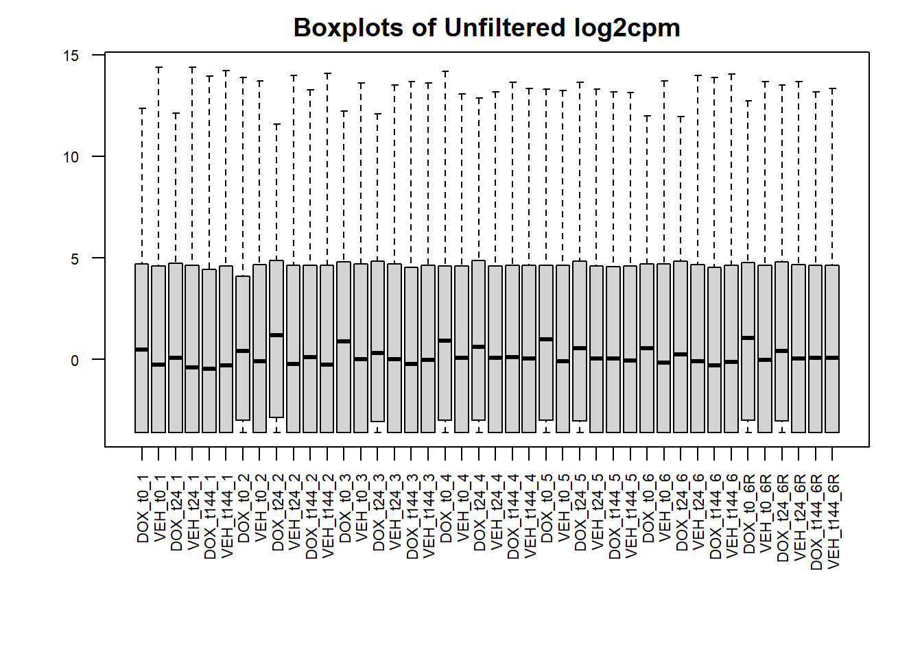
#set the margins so the x axis isn't cut off
par(mar = c(8,4,2,2))
#boxplot of filtered cpm matrix
boxplot(filcpm_matrix,
        main = "Boxplots of Filtered log2cpm (rowMeans > 0)",
        names = colnames(filcpm_matrix),
        adj=1, las = 2, cex.axis = 0.7)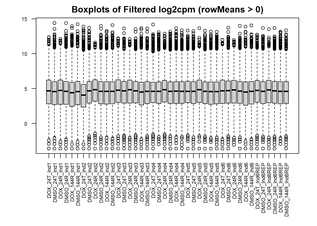
| Version | Author | Date |
|---|---|---|
| a967d53 | emmapfort | 2025-12-09 |
Add HGNC SYMBOL to final dataframe
##I did this earlier so don't run again, I put the list into the filcpm_final_matrix.csv (also already changed 84-1 to 4)
#load in my data
# sample_data <- read.csv("data/new/filcpm_final_matrix.csv")
#ensure Entrez_ID is present and in character Format
# Check column names
# print(colnames(sample_data))
# # Rename if needed (adjust if the column name is not exactly 'Entrez_ID')
# sample_data <- sample_data %>% dplyr::rename(Entrez_ID = "X")
# # Convert Entrez_ID to character
# sample_data <- sample_data %>%
# mutate(Entrez_ID = as.character(Entrez_ID))
# ----------------- Map Entrez_ID to Gene Symbol -----------------
# gene_symbols <- AnnotationDbi::select(
# org.Hs.eg.db,
# keys = sample_data$Entrez_ID,
# columns = c("SYMBOL"),
# keytype = "ENTREZID"
# )
# ----------------- Join Back to Main Data -----------------
# sample_annotated <- left_join(sample_data, gene_symbols, by = c("Entrez_ID" = "ENTREZID"))
# ----------------- Save Annotated Output -----------------
# write_csv(sample_annotated, "data/Sample_annotated.csv")
#Since I ran this before, Sample_annotated.csv columns of EntrezID and Symbol have been copied into my final matrix boxplot1 - so disregard this file except for record-keeping
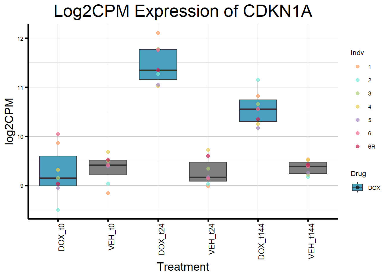
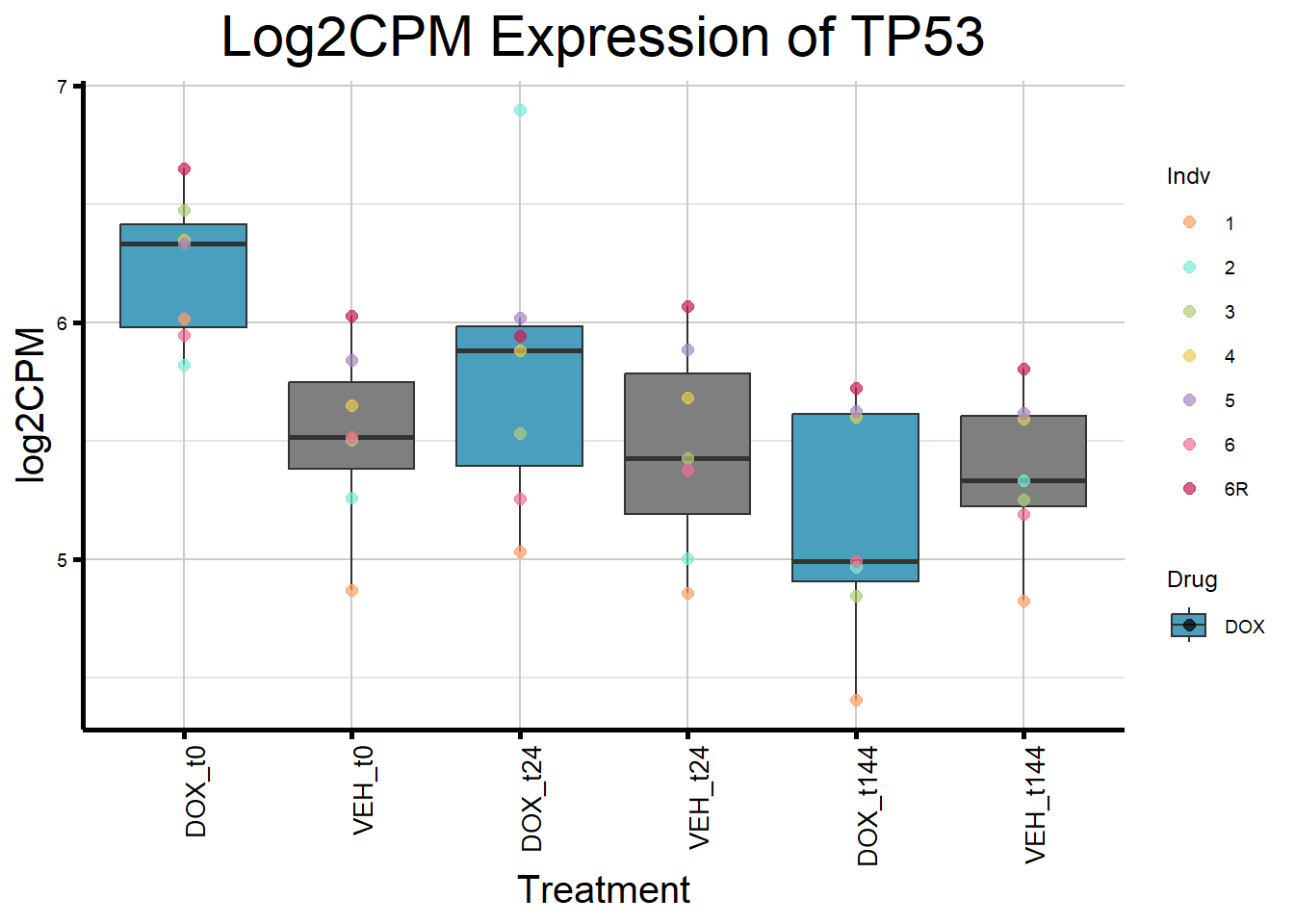
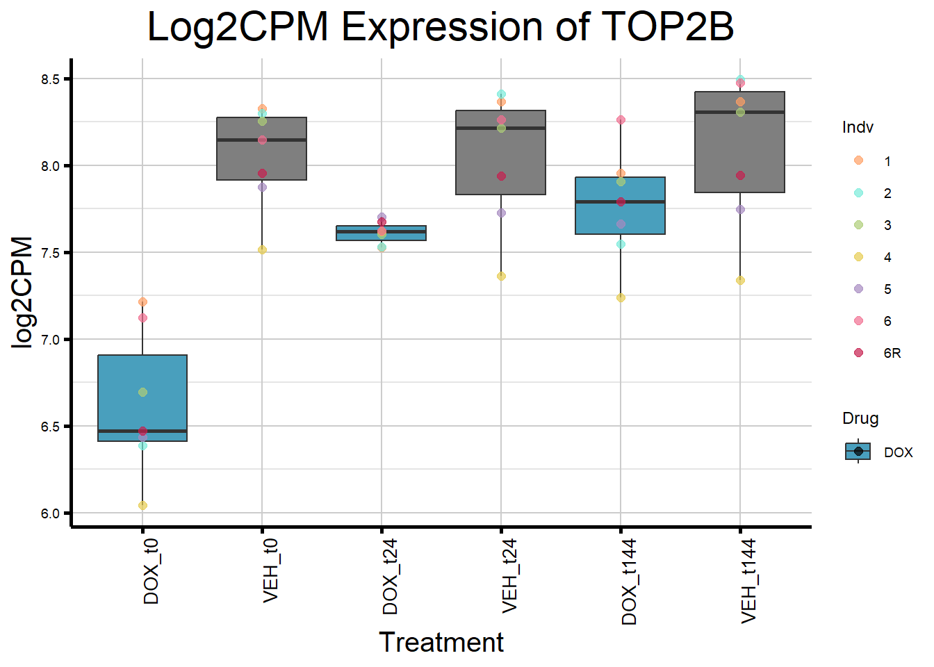
# saveRDS(boxplot1, "data/QC/filcpm_matrix_genes.RDS")Check Response Genes log2cpm
#get object from above that is now boxplot1
boxplot1 <- readRDS("data/QC/filcpm_matrix_genes.RDS")
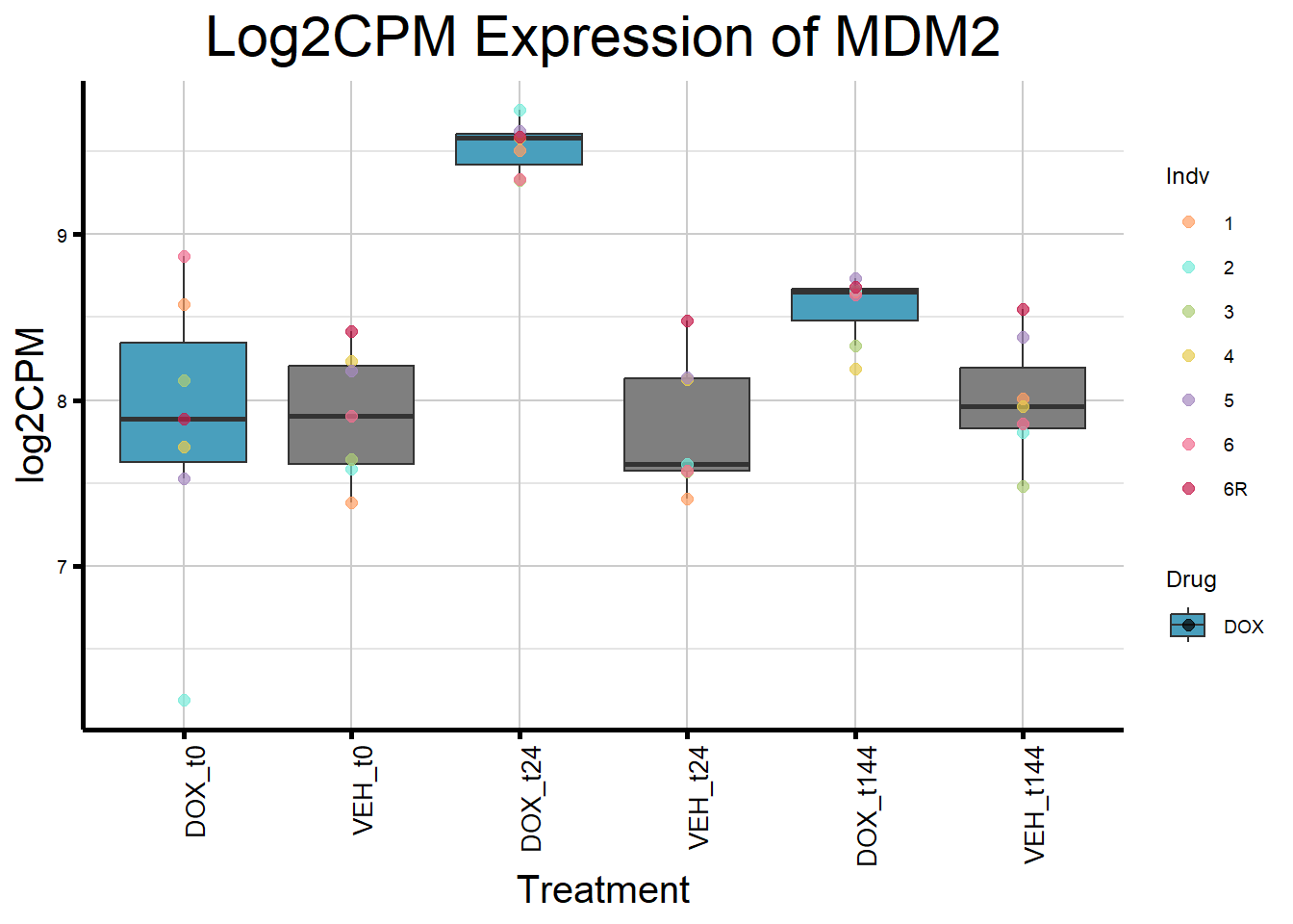
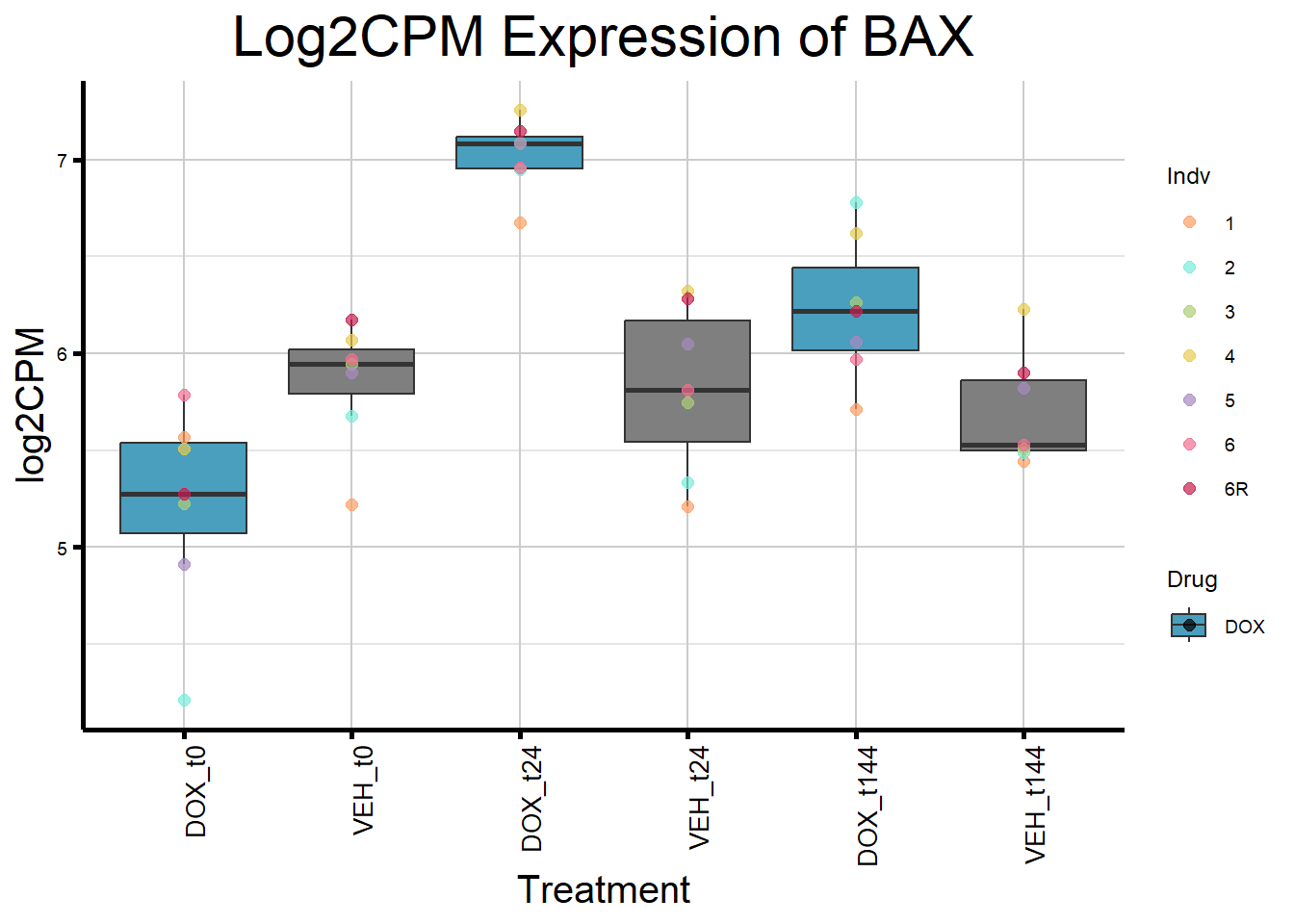
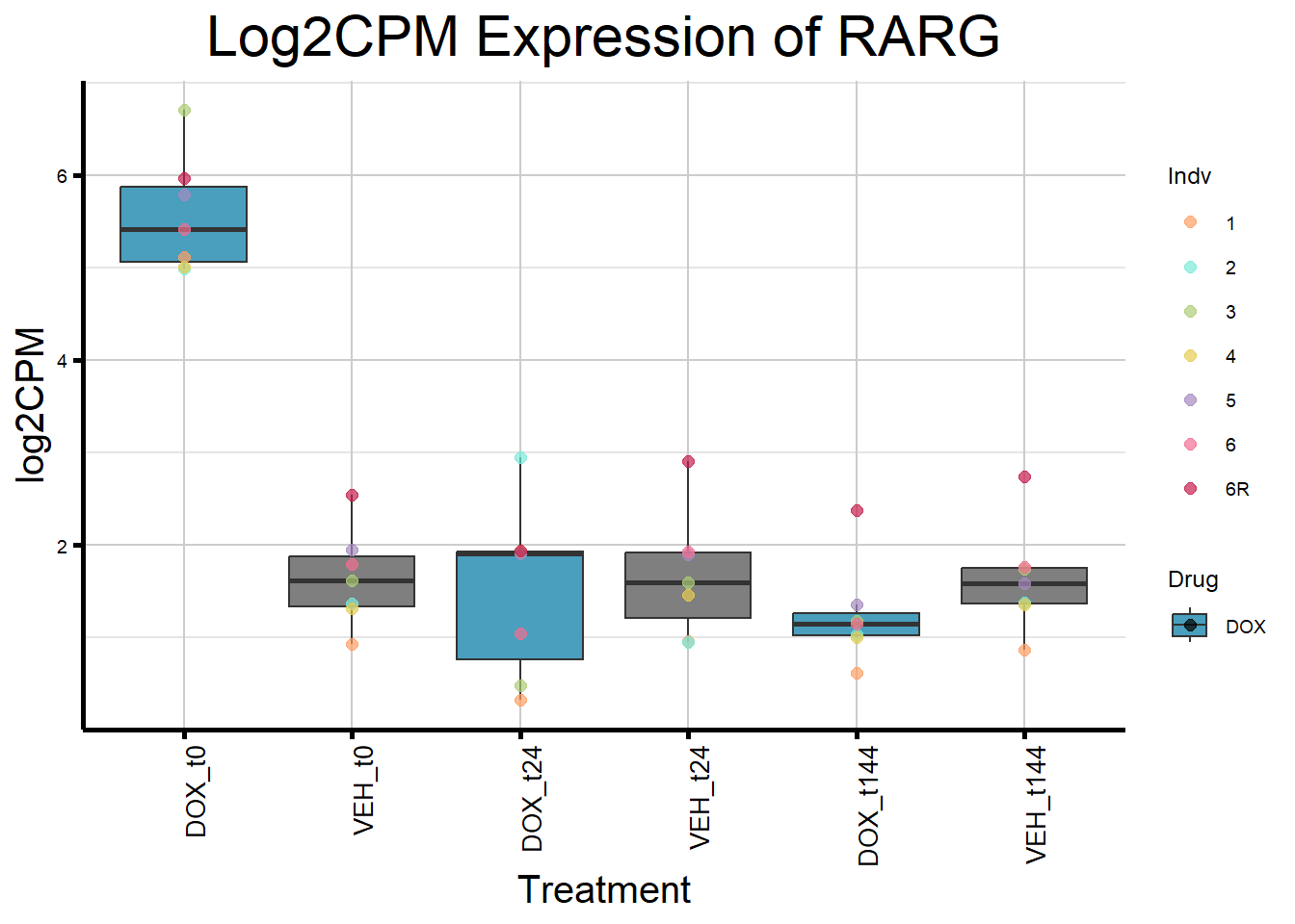
#Define gene list(s)
initial_test_genes <- c("CDKN1A", "MDM2", "BAX", "RARG", "TP53", "TOP2B")
#Add more gene symbols as needed or add more categories
#Now put in the function I want to use to generate boxplots of genes
process_gene_data <- function(gene) {
gene_data <- boxplot1 %>% filter(SYMBOL == gene)
long_data <- gene_data %>%
pivot_longer(cols = -c(Entrez_ID, SYMBOL), names_to = "Sample", values_to = "log2CPM") %>%
mutate(
Drug = case_when(
grepl("DOX", Sample) ~ "DOX",
grepl("DMSO", Sample) ~ "VEH",
TRUE ~ NA_character_
),
Timepoint = case_when(
grepl("_24T_", Sample) ~ "t0",
grepl("_24R_", Sample) ~ "t24",
grepl("_144R_", Sample) ~ "t144",
TRUE ~ NA_character_
),
Indv = case_when(
grepl("Ind1$", Sample) ~ "1",
grepl("Ind2$", Sample) ~ "2",
grepl("Ind3$", Sample) ~ "3",
grepl("Ind4$", Sample) ~ "4",
grepl("Ind5$", Sample) ~ "5",
grepl("Ind6$", Sample) ~ "6",
grepl("Ind6REP$", Sample) ~ "6R",
TRUE ~ NA_character_
),
Condition = paste(Drug, Timepoint, sep = "_")
)
long_data$Condition <- factor(
long_data$Condition,
levels = c(
"DOX_t0",
"VEH_t0",
"DOX_t24",
"VEH_t24",
"DOX_t144",
"VEH_t144"
)
)
return(long_data)
}
#this function is saved under process_gene_data so I will save as an R object
# saveRDS(process_gene_data, "data/funct/process_gene_data_funct.RDS")
#Generate Boxplots from the above function using our gene list above
for (gene in initial_test_genes) {
gene_data <- process_gene_data(gene)
gene_plots <- ggplot(gene_data, aes(x = Condition, y = log2CPM, fill = Drug)) +
geom_boxplot(outlier.shape = NA) +
geom_point(aes(color = Indv), size = 2, alpha = 0.7, position = position_identity()) +
scale_fill_manual(values = c("DOX" = "#499FBD", "DMSO" = "#BBBBBC")) +
scale_color_manual(values = ind_col) +
ggtitle(paste("Log2CPM Expression of", gene)) +
labs(x = "Treatment", y = "log2CPM") +
theme_custom() +
theme(
plot.title = element_text(size = rel(2), hjust = 0.5),
axis.title = element_text(size = 15, color = "black"),
axis.text.x = element_text(size = 10, color = "black", angle = 90, hjust = 1)
)
print(gene_plots)
}
| Version | Author | Date |
|---|---|---|
| a967d53 | emmapfort | 2025-12-09 |
| Version | Author | Date |
|---|---|---|
| a967d53 | emmapfort | 2025-12-09 |
| Version | Author | Date |
|---|---|---|
| a967d53 | emmapfort | 2025-12-09 |
| Version | Author | Date |
|---|---|---|
| a967d53 | emmapfort | 2025-12-09 |
| Version | Author | Date |
|---|---|---|
| a967d53 | emmapfort | 2025-12-09 |
| Version | Author | Date |
|---|---|---|
| a967d53 | emmapfort | 2025-12-09 |
sessionInfo()R version 4.4.2 (2024-10-31 ucrt)
Platform: x86_64-w64-mingw32/x64
Running under: Windows 11 x64 (build 22000)
Matrix products: default
locale:
[1] LC_COLLATE=English_United States.utf8
[2] LC_CTYPE=English_United States.utf8
[3] LC_MONETARY=English_United States.utf8
[4] LC_NUMERIC=C
[5] LC_TIME=English_United States.utf8
time zone: America/Chicago
tzcode source: internal
attached base packages:
[1] grid stats graphics grDevices utils datasets methods
[8] base
other attached packages:
[1] ggrepel_0.9.6 ComplexHeatmap_2.22.0 ggfortify_0.4.17
[4] edgeR_4.4.0 limma_3.62.1 readxl_1.4.5
[7] lubridate_1.9.4 forcats_1.0.0 stringr_1.5.1
[10] dplyr_1.1.4 purrr_1.0.4 readr_2.1.5
[13] tidyr_1.3.1 tibble_3.2.1 ggplot2_3.5.2
[16] tidyverse_2.0.0 workflowr_1.7.1
loaded via a namespace (and not attached):
[1] tidyselect_1.2.1 farver_2.1.2 fastmap_1.2.0
[4] promises_1.3.2 digest_0.6.37 timechange_0.3.0
[7] lifecycle_1.0.4 cluster_2.1.6 statmod_1.5.0
[10] processx_3.8.6 magrittr_2.0.3 compiler_4.4.2
[13] rlang_1.1.6 sass_0.4.10 tools_4.4.2
[16] yaml_2.3.10 knitr_1.50 labeling_0.4.3
[19] RColorBrewer_1.1-3 withr_3.0.2 BiocGenerics_0.52.0
[22] stats4_4.4.2 git2r_0.36.2 colorspace_2.1-1
[25] scales_1.4.0 iterators_1.0.14 cli_3.6.3
[28] rmarkdown_2.29 crayon_1.5.3 generics_0.1.4
[31] rstudioapi_0.17.1 httr_1.4.7 tzdb_0.5.0
[34] rjson_0.2.23 cachem_1.1.0 parallel_4.4.2
[37] cellranger_1.1.0 matrixStats_1.5.0 vctrs_0.6.5
[40] jsonlite_2.0.0 callr_3.7.6 IRanges_2.40.0
[43] hms_1.1.3 GetoptLong_1.0.5 S4Vectors_0.44.0
[46] clue_0.3-66 locfit_1.5-9.12 foreach_1.5.2
[49] jquerylib_0.1.4 glue_1.8.0 codetools_0.2-20
[52] ps_1.9.1 stringi_1.8.7 gtable_0.3.6
[55] shape_1.4.6.1 later_1.4.2 pillar_1.10.2
[58] htmltools_0.5.8.1 circlize_0.4.16 R6_2.6.1
[61] doParallel_1.0.17 rprojroot_2.0.4 evaluate_1.0.3
[64] lattice_0.22-6 png_0.1-8 httpuv_1.6.16
[67] bslib_0.9.0 Rcpp_1.0.14 gridExtra_2.3
[70] whisker_0.4.1 xfun_0.52 fs_1.6.6
[73] getPass_0.2-4 pkgconfig_2.0.3 GlobalOptions_0.1.2